Download Excel 2010 Expert.77-888.BrainDumps.2018-12-21.35q.vcex
| Vendor: | Microsoft |
| Exam Code: | 77-888 |
| Exam Name: | Excel 2010 Expert |
| Date: | Dec 21, 2018 |
| File Size: | 2 MB |
How to open VCEX files?
Files with VCEX extension can be opened by ProfExam Simulator.
Discount: 20%
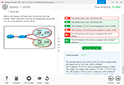

Demo Questions
Question 1
You work as an Office Assistant for Blue well Inc. The company has a Windows-based network. You want to create a VBA procedure for the open event of a workbook. You are at the step of adding the following lines of code to the procedure:
"Private Sub Workbook_Open() MsgBox Time Worksheets("Sheet2").Range("A2").Value = Time End Sub"
Which of the following are the next steps that you will take to accomplish the task? Each correct answer represents a part of the solution. Choose all that apply.
- Under Macro Settings in the Macro Settings category, click Enable all macros, and then click OK.
- Switch to Excel and save the workbook with the .xslm extension as a macro-enabled workbook and close it.
- Reopen the workbook.
- Click OK in the message box.
Correct answer: BCD
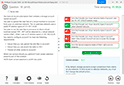
Question 2
Which of the following steps will you take to merge copies of a shared workbook? Each correct answer represents a part of the solution. Choose all that apply.
- In the Select Files to Merge into Current Workbook dialog box, click a copy of the workbook containing changes to be merged, and then click OK.
- Click Compare and Merge Workbooks on Quick Access Toolbar.
- Open the copy of the shared workbook to merge the changes.
- Save the workbook if prompted.
- Add Compare and Merge Workbooks.
- Click Compare and Merge Workbooks on Macro Enabled Access Toolbar.
Correct answer: ABCDE
Explanation:
Take the following steps to merge copies of a shared workbook:Add Compare and Merge Workbooks. Open the copy of the shared workbook to merge the changes. Click Compare and Merge Workbooks on Quick Access Toolbar. Save the workbook if prompted. In the Select Files to Merge into Current Workbook dialog box, click a copy of the workbook containing changes to be merged, and then click OK. Take the following steps to merge copies of a shared workbook:
- Add Compare and Merge Workbooks.
- Open the copy of the shared workbook to merge the changes.
- Click Compare and Merge Workbooks on Quick Access Toolbar.
- Save the workbook if prompted.
- In the Select Files to Merge into Current Workbook dialog box, click a copy of the workbook containing changes to be merged, and then click OK.
Question 3
You work as an Office Assistant for Blue Well Inc. The company has a Windows-based network. Some employees have changed some data in the worksheet of the company. You want to identify changes that were made to the data in the workbook and then take a decision whether to accept or reject those changes. For this purpose, it is required to access and use the stored change history.
Which of the following will you use to accomplish the task?
Each correct answer represents a complete solution. Choose all that apply.
- History tracking
- Onscreen highlighting
- Slicer-enabled highlighting
- Reviewing of changes
Correct answer: ABD
Explanation:
The following ways are provided by Excel to access and use the stored change history:Onscreen highlighting: It is used when a workbook does not contain many changes and a user wants to see all changes at a glance.History tracking: It is used when a workbook has many changes and a user wants to investigate what occurred in a series of changes.Reviewing of changes: It is used when a user is evaluating comments from other users. Answer option C is incorrect. This is an invalid answer option. The following ways are provided by Excel to access and use the stored change history:
- Onscreen highlighting: It is used when a workbook does not contain many changes and a user wants to see all changes at a glance.
- History tracking: It is used when a workbook has many changes and a user wants to investigate what occurred in a series of changes.
- Reviewing of changes: It is used when a user is evaluating comments from other users. Answer option C is incorrect. This is an invalid answer option.
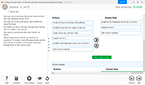
Question 4
You work as a Sales Manager for Tech Perfect Inc. You are creating a report for your sales team Using Microsoft Excel. You want the report to appear in the following format:

You want the Remark column to be filled through a conditional formula. The criteria to give the remark is as follows:
- If the sales of the First Quarter are greater than or equal to 1200, display "Well Done"
- If the sales of the First Quarter is less than 1200, display "Improve in Next Quarter"
You have done most of the entries in a workbook. You select the F2 cell as shown in the image given below:

Which of the following conditional formulas will you insert to accomplish the task?
- =IF(E2>=1200,"Improve in Next Quarter","Well Done")
- =IF(E2<=1200,"Well Done","Improve in Next Quarter")
- =IF(E2>=1200,"Well Done","Improve in Next Quarter")
- =IF(E2>1200,"Improve in Next Quarter","Well Done")
Correct answer: C
Explanation:
In order to accomplish the task, you will have to insert the following formula in the F2 cell:=IF(E2>=1200,"Well Done","Improve in Next Quarter") Answer option A is incorrect. This will display the wrong messages for the given conditions. The first expression after the logical condition is returned by the IF function when the condition is TRUE. Answer option B is incorrect. This formula will not accomplish the task as the logical condition is not correct. The specified condition in this formula is testing for values less than or equal to 1200. Whereas, the question's requirement is to evaluate values greater than or equal to 1200. Answer option D is incorrect. This formula will not accomplish the task because of the two reasons. First, the equal sign is missing in the condition. Second, the expressions are not in the correct order. In order to accomplish the task, you will have to insert the following formula in the F2 cell:
=IF(E2>=1200,"Well Done","Improve in Next Quarter")
Answer option A is incorrect. This will display the wrong messages for the given conditions. The first expression after the logical condition is returned by the IF function when the condition is TRUE.
Answer option B is incorrect. This formula will not accomplish the task as the logical condition is not correct. The specified condition in this formula is testing for values less than or equal to 1200. Whereas, the question's requirement is to evaluate values greater than or equal to 1200.
Answer option D is incorrect. This formula will not accomplish the task because of the two reasons.
First, the equal sign is missing in the condition. Second, the expressions are not in the correct order.
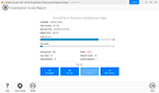
Question 5
You work as an Office Assistant for Peach Tree Inc. Your responsibility includes creating sales incentive report of all sales managers for every quarter. You are using Microsoft Excel to create a worksheet for preparing the report. You have inserted the sales figures of all sales managers as shown in the image given below:

You have to calculate the first quarter incentives for all sales managers. The incentive percentage (provided in cell B3) is fixed for all sales managers. The incentive will be calculated on their total first quarter sales. You have to write a formula in the cell F8. Then you will drag the cell border to the cell F12 to copy the formula to all the cells from F8 to F12. In the first step, you select the F8 cell. Which of the following formulas will you insert to accomplish the task?
- =&B&3/100 * E8
- =B3/100 * E8
- =B3/100 * &E&8
- =$B$3/100 * E8
- =B3/100 * $E$8
Correct answer: D
Explanation:
In order to accomplish the task, you will have to insert the following formula:=$B$3/100 * E8 According to the question, the formula will be inserted in cell F8 and then the cell's border will be dragged to the F12 cell. Furthermore, the incentive percentage is fixed for all sales managers and the value is provided in the cell B3. You will have to insert a formula that refers to the B3 cell as an absolute reference. For this you will have to type currency symbol ($) before the row name and column number. In order to accomplish the task, type the following formula in the cell F8:=$B$3/100 * E8 When absolute reference is used for referencing a cell in a formula, dragging cell's border to another cell does not change the cell's reference. Answer options B and E are incorrect. This formula references the B3 cell as a relative reference. After inserting the formula, when the cell's border is dragged, it will change the cell reference relatively. Answer options A and C are incorrect. Ampersand symbol (&) is not used for referencing cells in Excel. In order to accomplish the task, you will have to insert the following formula:
=$B$3/100 * E8
According to the question, the formula will be inserted in cell F8 and then the cell's border will be dragged to the F12 cell. Furthermore, the incentive percentage is fixed for all sales managers and the value is provided in the cell B3. You will have to insert a formula that refers to the B3 cell as an absolute reference. For this you will have to type currency symbol ($) before the row name and column number. In order to accomplish the task, type the following formula in the cell F8:
=$B$3/100 * E8
When absolute reference is used for referencing a cell in a formula, dragging cell's border to another cell does not change the cell's reference.
Answer options B and E are incorrect. This formula references the B3 cell as a relative reference.
After inserting the formula, when the cell's border is dragged, it will change the cell reference relatively.
Answer options A and C are incorrect. Ampersand symbol (&) is not used for referencing cells in Excel.
Question 6
You work as an Office Assistant for Dreams Unlimited Inc. You use Microsoft Excel 2010 for creating various types of reports. You have created a report in the format given below:

In the A7 cell, you are required to put a formula so that it can fulfill the description provided in the B7 cell.
Which of the following formulas will provide the required result?
- COUNTIF(B2:C5,"=Yes")
- COUNTIFS(B2:C5,"=Yes")
- COUNTIF(B2:B5,"=Yes",C2:C5,"=Yes")
- COUNTIFS(B2:B5,"=Yes",C2:C5,"=Yes")
Correct answer: D
Explanation:
In order to get the required result, you will have to insert the following formula in the B7 cell:COUNTIFS(B2:B5,"=Yes",C2:C5,"=Yes")Only Sarah and David have exceeded their January and February quotas, therefore the formula will provide 2 as the result. Answer option C is incorrect. The COUNTIF function of Excel does not support multiple criteria. Answer options A and B are incorrect. This formula will count all the cells that have the value "Yes" in the range B2:C5. As multiple criteria are not applied in the formula, it will provide 6 as the result. In order to get the required result, you will have to insert the following formula in the B7 cell:
COUNTIFS(B2:B5,"=Yes",C2:C5,"=Yes")
Only Sarah and David have exceeded their January and February quotas, therefore the formula will provide 2 as the result.
Answer option C is incorrect. The COUNTIF function of Excel does not support multiple criteria.
Answer options A and B are incorrect. This formula will count all the cells that have the value "Yes" in the range B2:C5. As multiple criteria are not applied in the formula, it will provide 6 as the result.
Question 7
You work as an Office Assistant for Media Perfect Inc. You have created a spreadsheet in Excel 2010 and shared it with the other employees of the company. You want to protect the worksheet and locked cells by permitting or prohibiting other employees to select, format, insert, delete, sort, or edit areas of the spreadsheet. Which of the following options will you use to accomplish the task?
- Mark as Final
- Encrypt with Password
- Protect Current Sheet
- Protect Workbook Structure
Correct answer: C
Explanation:
The various Protect Workbook options are as follows:Mark as Final: This option is used to make the document read-only. When a spreadsheet is marked as final, various options such as typing, editing commands, and proofing marks are disabled or turned off and the spreadsheet becomes read-only. This command helps a user to communicate that he is sharing a completed version of a spreadsheet. This command also prevents reviewers or readers from making inadvertent modifications to the spreadsheet.Encrypt with Password: When a user selects the Encrypt with Password option, the Encrypt Document dialog box appears. In the Password box, it is required to specify a password. Microsoft is not able to retrieve lost or forgotten passwords, so it is necessary for a user to keep a list of passwords and corresponding file names in a safe place.Protect Current Sheet: This option is used to select password protection and permit or prohibit other users to select, format, insert, delete, sort, or edit areas of the spreadsheet. This option protects the worksheet and locked cells.Protect Workbook Structure: This option is used to select password protection and select options to prevent users from changing, moving, and deleting important data. This feature enables a user to protect the structure of the worksheet.Restrict Permission by People: This option works on the basis of Window Rights Management to restrict permissions. A user is required to use a Windows Live ID or a Microsoft Windows account to restrict permissions. These permissions can be applied via a template that is used by the organization in which the user is working. These permissions can also be added by clicking Restrict Access.Add a Digital Signature: This option is used to add a visible or invisible digital signature. It authenticates digital information such as documents, e-mail messages, and macros by using computer cryptography. These signatures are created by specifying a signature or by using an image of a signature for establishing authenticity, integrity, and non-repudiation. The various Protect Workbook options are as follows:
- Mark as Final: This option is used to make the document read-only. When a spreadsheet is marked as final, various options such as typing, editing commands, and proofing marks are disabled or turned off and the spreadsheet becomes read-only. This command helps a user to communicate that he is sharing a completed version of a spreadsheet. This command also prevents reviewers or readers from making inadvertent modifications to the spreadsheet.
- Encrypt with Password: When a user selects the Encrypt with Password option, the Encrypt Document dialog box appears. In the Password box, it is required to specify a password. Microsoft is not able to retrieve lost or forgotten passwords, so it is necessary for a user to keep a list of passwords and corresponding file names in a safe place.
- Protect Current Sheet: This option is used to select password protection and permit or prohibit other users to select, format, insert, delete, sort, or edit areas of the spreadsheet. This option protects the worksheet and locked cells.
- Protect Workbook Structure: This option is used to select password protection and select options to prevent users from changing, moving, and deleting important data. This feature enables a user to protect the structure of the worksheet.
- Restrict Permission by People: This option works on the basis of Window Rights Management to restrict permissions. A user is required to use a Windows Live ID or a Microsoft Windows account to restrict permissions. These permissions can be applied via a template that is used by the organization in which the user is working. These permissions can also be added by clicking Restrict Access.
- Add a Digital Signature: This option is used to add a visible or invisible digital signature. It authenticates digital information such as documents, e-mail messages, and macros by using computer cryptography. These signatures are created by specifying a signature or by using an image of a signature for establishing authenticity, integrity, and non-repudiation.

Question 8
Rick works as an Office Assistant for Tech Perfect Inc. He is creating a user form through Microsoft Excel 2010. While creating forms for a number of users, he is required to repeat some of the actions multiple times. It is a very time consuming process. To resolve the issue, he has created a macro to record the sequence of actions to perform a certain task. Now, he wants to run the macro to play those exact actions back in the same order. Which of the following steps will Rick take to accomplish the task?
Each correct answer represents a part of the solution. Choose all that apply.
- Click on the 'Macros' icon in the 'Developer' tab under the 'Code' category to run a Macro.
- The Macro will be run in any worksheet of the Workbook.
- Put the workbook in a trusted location.
- The Macro dialogue box appears on the screen which contains a list of Macros in it. Select the Macro to run and click the Run button.
- Run the created Macro by using the shortcut key specified while creating the Macro.
Correct answer: ABDE
Explanation:
Take the following steps to run a Macro:1. Click on the 'Macros' icon in the 'Developer' tab under the 'Code' category to run a Macro. 2. The Macro dialogue box appears on the screen which contains a list of Macros in it. Select the Macro to run and click the Run button. 3. The Macro will be run in any worksheet of the Workbook. 4. A user can run the created Macro by using the shortcut key that he has specified while creating the Macro. The macro records the user's mouse clicks and keystrokes while he works and lets him play them back later. The macro can be used to record the sequence of commands that the user uses to perform a certain task. When the user runs the macro, it plays those exact commands back in the same order. Answer option C is incorrect. The benefit of connecting to external data from Microsoft Excel is that a user can automatically update Excel workbooks from the real data source whenever the data source is updated with new information. It is possible that the external data connection might be disabled on the computer. For connecting to the data source whenever a workbook is opened, it is required to enable data connections by using the Trust Center bar or by putting the workbook in a trusted location. Take the following steps to run a Macro:
1. Click on the 'Macros' icon in the 'Developer' tab under the 'Code' category to run a Macro.

2. The Macro dialogue box appears on the screen which contains a list of Macros in it. Select the Macro to run and click the Run button.

3. The Macro will be run in any worksheet of the Workbook.
4. A user can run the created Macro by using the shortcut key that he has specified while creating the Macro. The macro records the user's mouse clicks and keystrokes while he works and lets him play them back later. The macro can be used to record the sequence of commands that the user uses to perform a certain task. When the user runs the macro, it plays those exact commands back in the same order. Answer option C is incorrect. The benefit of connecting to external data from Microsoft Excel is that a user can automatically update Excel workbooks from the real data source whenever the data source is updated with new information. It is possible that the external data connection might be disabled on the computer. For connecting to the data source whenever a workbook is opened, it is required to enable data connections by using the Trust Center bar or by putting the workbook in a trusted location.
Question 9
You work as an Office Assistant for Tech Perfect Inc. You are working in a spreadsheet. You are facing a problem that when you type in a function and press Enter, the cell shows the function as you typed it, instead of returning the function's value as shown below:
Which of the following is the reason that is causing the above problem?
- You are inserting a new column, next to a column that is already formatted as text.
- Excel is trying to reference an invalid cell.
- You are inserting a new column, next to a column containing Dates or Times.
- The lookup_value or the array you are searching resides in a cell containing unseen spaces at the start or end of that cell.
Correct answer: A
Explanation:
The Excel Won't Calculate My Function error occurs when a user types in a function and presses Enter, the cell shows the function as the user typed it, instead of returning the function's value. The reason that causes this problem is that the cells containing the formula are formatted as 'text' instead of the 'General' type. This happens when the user inserts a new column, next to a column that is already formatted as text due to which the new column inherits the formatting of the adjacent column. Answer option D is incorrect. The Failure to Look Up Values in Excel error occurs when a user gets an unexpected error while trying to look up or match a lookup_value within an array and Excel is not able to recognize the matching value. If the lookup_value or the array the user is searching resides in a cell, the user can have unseen spaces at the start or end of that cell. This will create the situation where the contents of the two cells that the user is comparing look the same but extra spaces in one of the cells cause the cells to have slightly different content. The other reason is that the contents of the cells that are being compared may have different data types. Answer option B is incorrect. The Lookup Function Won't Copy Down to Other Rows error occurs when a user uses a function in one cell and it works perfectly but when he attempts to copy the function down to other rows, he gets the #REF error. The #REF! error arises when Excel tries to reference an invalid cell. This error occurs if the user has referenced an entire worksheet by clicking on the grey square at the top left of the worksheet. For Excel, this reference range is 1 to 1048576. Since the references are Relative References, Excel automatically increases the row references when this cell is copied down to other rows in the spreadsheet. Answer option C is incorrect. The Cell Shows a Date or Time Instead of a Number error occurs because the cell that contains the formula is formatted as a 'date' or 'time' instead of a 'General' type or a number. This situation arises because a user has inserted a new column, next to a column containing Dates or Times, the new column has 'inherited' the formatting of the adjacent column. The Excel Won't Calculate My Function error occurs when a user types in a function and presses Enter, the cell shows the function as the user typed it, instead of returning the function's value.
The reason that causes this problem is that the cells containing the formula are formatted as 'text' instead of the 'General' type. This happens when the user inserts a new column, next to a column that is already formatted as text due to which the new column inherits the formatting of the adjacent column. Answer option D is incorrect. The Failure to Look Up Values in Excel error occurs when a user gets an unexpected error while trying to look up or match a lookup_value within an array and Excel is not able to recognize the matching value. If the lookup_value or the array the user is searching resides in a cell, the user can have unseen spaces at the start or end of that cell. This will create the situation where the contents of the two cells that the user is comparing look the same but extra spaces in one of the cells cause the cells to have slightly different content. The other reason is that the contents of the cells that are being compared may have different data types.
Answer option B is incorrect. The Lookup Function Won't Copy Down to Other Rows error occurs when a user uses a function in one cell and it works perfectly but when he attempts to copy the function down to other rows, he gets the #REF error. The #REF! error arises when Excel tries to reference an invalid cell. This error occurs if the user has referenced an entire worksheet by clicking on the grey square at the top left of the worksheet. For Excel, this reference range is 1 to 1048576. Since the references are Relative References, Excel automatically increases the row references when this cell is copied down to other rows in the spreadsheet. Answer option C is incorrect. The Cell Shows a Date or Time Instead of a Number error occurs because the cell that contains the formula is formatted as a 'date' or 'time' instead of a 'General' type or a number. This situation arises because a user has inserted a new column, next to a column containing Dates or Times, the new column has 'inherited' the formatting of the adjacent column.
Question 10
You work as an Office Assistant for Media Perfect Inc. You have created a spreadsheet in Excel 2010 and shared it with the other employees of the company. You want to select password protection and select options to prevent other employees from changing, moving, and deleting important data.
Which of the following options will you choose to accomplish the task?
- Mark as Final
- Protect Current Sheet
- Encrypt with Password
- Protect Workbook Structure
Correct answer: D
Explanation:
The various Protect Workbook options are as follows:Mark as Final: This option is used to make the document read-only. When a spreadsheet is marked as final, various options such as typing, editing commands, and proofing marks are disabled or turned off and the spreadsheet becomes read-only. This command helps a user to communicate that he is sharing a completed version of a spreadsheet. This command also prevents reviewers or readers from making inadvertent modifications to the spreadsheet.Encrypt with Password: When a user selects the Encrypt with Password option, the Encrypt Document dialog box appears. In the Password box, it is required to specify a password. Microsoft is not able to retrieve lost or forgotten passwords, so it is necessary for a user to keep a list of passwords and corresponding file names in a safe place.Protect Current Sheet: This option is used to select password protection and permit or prohibit other users to select, format, insert, delete, sort, or edit areas of the spreadsheet. This option protects the worksheet and locked cells.Protect Workbook Structure: This option is used to select password protection and select options to prevent users from changing, moving, and deleting important data. This feature enables a user to protect the structure of the worksheet.Restrict Permission by People: This option works on the basis of Window Rights Management to restrict permissions. A user is required to use a Windows Live ID or a Microsoft Windows account to restrict permissions. These permissions can be applied via a template that is used by the organization in which the user is working. These permissions can also be added by clicking Restrict Access.Add a Digital Signature: This option is used to add a visible or invisible digital signature. It authenticates digital information such as documents, e-mail messages, and macros by using computer cryptography. These signatures are created by specifying a signature or by using an image of a signature for establishing authenticity, integrity, and non-repudiation. The various Protect Workbook options are as follows:
- Mark as Final: This option is used to make the document read-only. When a spreadsheet is marked as final, various options such as typing, editing commands, and proofing marks are disabled or turned off and the spreadsheet becomes read-only. This command helps a user to communicate that he is sharing a completed version of a spreadsheet. This command also prevents reviewers or readers from making inadvertent modifications to the spreadsheet.
- Encrypt with Password: When a user selects the Encrypt with Password option, the Encrypt Document dialog box appears. In the Password box, it is required to specify a password. Microsoft is not able to retrieve lost or forgotten passwords, so it is necessary for a user to keep a list of passwords and corresponding file names in a safe place.
- Protect Current Sheet: This option is used to select password protection and permit or prohibit other users to select, format, insert, delete, sort, or edit areas of the spreadsheet. This option protects the worksheet and locked cells.
- Protect Workbook Structure: This option is used to select password protection and select options to prevent users from changing, moving, and deleting important data. This feature enables a user to protect the structure of the worksheet.
- Restrict Permission by People: This option works on the basis of Window Rights Management to restrict permissions. A user is required to use a Windows Live ID or a Microsoft Windows account to restrict permissions. These permissions can be applied via a template that is used by the organization in which the user is working. These permissions can also be added by clicking Restrict Access.
- Add a Digital Signature: This option is used to add a visible or invisible digital signature. It authenticates digital information such as documents, e-mail messages, and macros by using computer cryptography. These signatures are created by specifying a signature or by using an image of a signature for establishing authenticity, integrity, and non-repudiation.
HOW TO OPEN VCE FILES
Use VCE Exam Simulator to open VCE files
HOW TO OPEN VCEX AND EXAM FILES
Use ProfExam Simulator to open VCEX and EXAM files

ProfExam at a 20% markdown
You have the opportunity to purchase ProfExam at a 20% reduced price
Get Now!